Geospatial exposure modeling methods and applications in human health

Kyle P Messier, PhD

Stadtman Tenure Track Investigator

National Institute of Environmental Health Sciences

Division of Translational Toxicology

ENVR 500 Guest Lecture: February 22, 2024

About Me

BS Environmental Science: UNC-Asheville
MS, PhD, Environmental Science and Engineering, UNC ESE, Advisor: Marc Serre
Postdoc, Environmental Defense Fund, High-Resolution Air Pollution Mapping with Mobile Monitoring
Research Faculty, Oregon State University, Department of Environmental and Molecular Toxicology
Tenure Track Investigator, NIH/NIEHS/DTT

About Us: {SET}_group

Spatiotemporal Exposure Mapping
Chemical and Stressor Mixtures Prediction
Mechanistically Informed Risk Assessment

About Us: {SET}_group

Eva Marques
Daniel Zilber
Ranadeep Daw
Mariana Alifa
Insang Song
Kyle Messier
Mitchell Manware (Not Pictured)

The Importance of Place

Hurricane Matthew, 2016
Hurricane Florence, 2018
Swine Waste Concerns
Fecal Bateria
Nitrate and Phosphorous Pollution
Infectious Diseases

History of Spatial [Geo] Statistics Mining

Matheron and Krige developed geostatistical methods to predict ore content from core samples
Matheron coined the term “Kriging” after Krige
“Nugget” is a term used to random noise because predicting where gold nuggets were was so difficult

History of Spatial [Geo] Statistics: Forestry

Matérn developed correlation models for spatial variation for applications in Forestry
To this day, we use the “Matérn” covariance function

History of Spatial [Geo] Statistics: Petroleum Engineering

Used to evaluate the oil and gas field reservoirs
Uses geology and seismic data

History of Spatial [Geo] Statistics: Public Health

Cressie, 1990: Statistics for Spatial Data
Waller and Gotway, 2004: Applied Statistics for Public Health Data
Wide scale adoption for statisticians and engineers in ecological and human exposure and risk applications

Source and Receptor Geometries

Questions:

In figure C, what is an example of geospatial health data geometry at a point? Check all that apply.
In figure I, what is an example of geospatial health data geometry at an area? Check all that apply.

Geospatial Health Analysis Overview

graph TD;

    style A fill:#91bcfd , stroke:#333, stroke-width:2px, rounded:true;
    style B fill:#91bcfd , stroke:#333, stroke-width:2px, rounded:true;
    style C fill:#91bcfd , stroke:#333, stroke-width:2px, rounded:true;

    A[Research Question: Exposure and Health Outcome Relationship?] --> B[Preparation of Geospatial Exposure Data];
    A --> C[Preparation of Health Outcome Data];

Geospatial Health Analysis Overview

graph TD;

    style A fill:#91bcfd , stroke:#333, stroke-width:2px, rounded:true;
    style B fill:#91bcfd , stroke:#333, stroke-width:2px, rounded:true;
    style C fill:#91bcfd , stroke:#333, stroke-width:2px, rounded:true;

    A[Research Question: Exposure and Health Outcome Relationship?] --> B[Preparation of Geospatial Exposure Data];
    A --> C[Preparation of Health Outcome Data];
    
    B1[Selection of Exposure Metrics];
    B2[Geospatial Exposure Modeling Strategy];
    B3[Geospatial data collection and integration];
    B4[Geospatial model fitting and calibration];
    

    B --> B1;
    B1 --> B2;
    B2 --> B3;
    B3 --> B4;

Questions:

what is an example of a point-level exposure data set? Check all that apply.
Which of the following are examples of an area-level exposure data set? Check all that apply.

Geospatial Health Analysis Overview

graph TD;

    style A fill:#91bcfd , stroke:#333, stroke-width:2px, rounded:true;
    style B fill:#91bcfd , stroke:#333, stroke-width:2px, rounded:true;
    style C fill:#91bcfd , stroke:#333, stroke-width:2px, rounded:true;

    A[Research Question: Exposure and Health Outcome Relationship?] --> B[Preparation of Geospatial Exposure Data];
    A --> C[Preparation of Health Outcome Data];
    
    B1[Selection of Exposure Metrics];
    B2[Geospatial Exposure Modeling Strategy];
    B3[Geospatial data collection and integration];
    B4[Geospatial model fitting and calibration];
    
    C1[Selection of health outcome metrics];
    C2[Health outcome data collection and integration: Individual or Population Level];
    C3[Geocoding of Health Outcome Data];

    B --> B1;
    B1 --> B2;
    B2 --> B3;
    B3 --> B4;
    
    C --> C1;
    C1 --> C2;
    C2 --> C3;

Geospatial Health Analysis Overview

graph TD;

    style A fill:#91bcfd , stroke:#333, stroke-width:2px, rounded:true;
    style B fill:#91bcfd , stroke:#333, stroke-width:2px, rounded:true;
    style C fill:#91bcfd , stroke:#333, stroke-width:2px, rounded:true;
    style D fill:#91bcfd , stroke:#333, stroke-width:2px, rounded:true;

    A[Research Question: Exposure and Health Outcome Relationship?] --> B[Preparation of Geospatial Exposure Data];
    A --> C[Preparation of Health Outcome Data];
    
    B1[Selection of Exposure Metrics];
    B2[Geospatial Exposure Modeling Strategy];
    B3[Geospatial data collection and integration];
    B4[Geospatial model fitting and calibration];
    
    C1[Selection of health outcome metrics];
    C2[Health outcome data collection and integration: Individual or Population Level];
    C3[Geocoding of Health Outcome Data];
    
    D[Exposure and Health Outcome Data Integration and Analysis];
    D1[Linkage of Exposure Model with Health Data];
    D2[Prediction of Exposure Model at Health Data Locations];
    D3[Exposure and Health Outcome Model Analysis];
    
    B --> B1;
    B1 --> B2;
    B2 --> B3;
    B3 --> B4;
    
    C --> C1;
    C1 --> C2;
    C2 --> C3;
    
    B4 --> D;
    C3 --> D;
    
    D --> D1;
    D1 --> D2;
    D2 --> D3;

The Landscape of Geospatial Exposure Models

The next section will focus on details of geospatial exposure models

Many types of models are used for geospatial exposure assessment.

Proximity
Index
Land Use Regression
Geographically Weighted Regression
Kriging and Gaussian Processes
Machine Learning
Mechanistic Models
Satellite Imagery
Hybrid / Ensemble Models

Notation: Spatial Random Field

\(\mathbf{y}\): A single random variable is denoted by a bold lowercase letter
\(\mathbf{Y}\): Spatial Random Field (SRF): A collection of random variables across a spatial domain.
SRF provides full, probabilistic characterization of exposure across space
SRF is referenced to a real-valued domain with spatial and temporal indices, \(\{\mathbf{Y}(s); s \in \mathbb{R}^2\}\).

A Review of Linear Regression

Response

\[ Y_i \in \{1, ..., n\} \] \(p\) covariates:

\[ X = X_{i1}, ..., X_{ip} \]

The model is :

\[ Y_i = \beta_0 + X_{i1}\beta_1 + , ..., X_{ip}\beta_p \]

The mean is a linear combination of the covariates

\[ E(Y_i) = \mu_i = \beta_0 + X_{i1}\beta_1 + ... + X_{ip}\beta_p \]

Error/Residuals are assumed to be independent and identically distributed (iid)

\[ \varepsilon_i = Y_i - \mu_i \]

Linear Regression for spatial idea

As a method, not a terrible idea
Unbiased
Overconfident error estiamte (p-values, SE)
Model Selection (Type 1 and 2 error)

Land Use Regression

Linear regression for spatial data

\[ \bY(s) = X(s)\beta + \varepsilon \]

\[ X(s) = X_{i1}(s_1), ..., X_{ip}(s_p) \]

Spatial Covariance Model

As a random-effect model, we add a spatially explicity error term

\[ \bY(s) = \mu(s) + \varepsilon + \eta(s) \]

\(\mu(s)\) can take many forms such as linear, nonlinear, or even machine learning models such as random forest.
More details on a spatial covariance model later

Proximity

Proximity based metrics are the most basic form of an exposure assessment because they rely only on the distance between a pollution source and the observed outcome location.
A proximity model is simply a deterministic covariate based on distance:

\[ Y(s) = X(s) \]

Given a matrix of distances between monitoring locations and pollution sources, \(d_{ij}\), minimum and average distance are:

\[ X_i^{min} = min(d_{i,\cdot}) \\ \overline{X}_i = \frac{1}{n_j}\sum_{j=1}^{n_j}d_{ij}\\ \]

Questions:

What are examples of proximity metrics? Check all that apply.
What are the advantages of a proximity metric? Check all that apply.

Index Models

Index variables are deterministic quantities that summarize (e.g. prinicipal components) multiple complex variables of interest into a simple and interpretable metric.
Covariates are made up of geographic variables across different domains
Social Vulnerability Index, Climate Vulnerability Index, etc.

Land Use Regression

\[ \bY(s) = X(s)\beta + \varepsilon \] - where \(\bY(p)\) are the \(n \times 1\) observations for the variable of interest (e.g. PM\(_{2.5}\), \(NO_3^{-}\), etc.). \(X(s)\) is a \(n \times k\) design matrix of \(k\) spatial geographic covariates

Key Steps

Calculate geographic covariates
Fit the model - may include model selection or dimension reduction
Predict at unmonitored locations

Geographically Weighted Regression

\[ \bY(s) = X(s)\beta(s) + \varepsilon \]
What is the key difference between LUR and GWR? Select one. Recall, LUR = \(\bY(s) = X(s)\beta + \varepsilon\)
Hint: It’s in the \(\beta\)

Gaussian Process and Kriging

Gaussian process and Kriging are one in the same
Utilize information on spatial correlation to help interpolate
Account for spatial error
Highly flexible

Gaussian Process and Kriging

\[ \bY(s) = \mu(s) + \eta(s) \]

\(\mu(s)\) can take many forms such as linear, nonlinear, or even machine learning models such as random forest
\(\eta \sim N_n(0,\Sigma_{\theta}+\tau^2I)\)
\(\Sigma_{\theta}\) is a covariance matrix with parameters, \(\theta\), that accounts for correlation between spatial and temporal locations

Question:

What physical quantity is \(\Sigma_{\theta}\) solely dependent on?

Machine Learning

Machine learning (ML) is the general culture, philosophy, or school of thought for predictive modeling that focuses on the learning algorithm and out-of-sample prediction generalization

Many common machine learning algorithms can be used for geospatial modeling
Flexible
Don’t make strict assumptions on the distriubtions of the data
Coordinates and other spatial information is input as covariates

Common Methods in Exposure Modeling

Generalized Additive Models (GAM)
Random Forest
xgboost
Neural Networks: CNN, LSTM, GAN, etc.

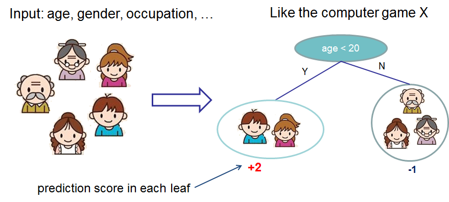
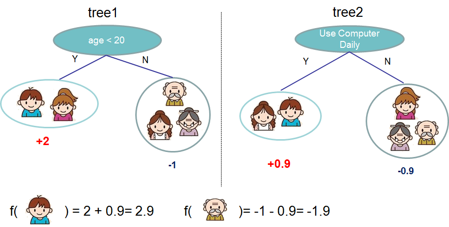
Machine Learning: Trees

Mechanistic

I would be remiss if I didn’t mention another entirely different class of exposure models
Mechanistic models are not statistical models
Mechanistic models are based on physics and chemistry

Hybrid

A consensus of multiple models is almost always better than any single model.

Requia, Weeberb J., et al. “An ensemble learning approach for estimating high spatiotemporal resolution of ground-level ozone in the contiguous United States.” Environmental science & technology 54.18 (2020): 11037-11047.

Yu, Wenhua, et al. “Deep ensemble machine learning framework for the estimation of PM 2.5 concentrations.” Environmental Health Perspectives 130.3 (2022): 037004.

Integrating Geospatial Exposure Models into Health Data

graph TD;

    style A fill:#91bcfd , stroke:#333, stroke-width:2px, rounded:true;
    style B fill:#91bcfd , stroke:#333, stroke-width:2px, rounded:true;
    style C fill:#91bcfd , stroke:#333, stroke-width:2px, rounded:true;
    style D fill:#91bcfd , stroke:#333, stroke-width:2px, rounded:true;

    A[Research Question: Exposure and Health Outcome Relationship?] --> B[Preparation of Geospatial Exposure Data];
    A --> C[Preparation of Health Outcome Data];
    
    B1[Selection of Exposure Metrics];
    B2[Geospatial Exposure Modeling Strategy];
    B3[Geospatial data collection and integration];
    B4[Geospatial model fitting and calibration];
    
    C1[Selection of health outcome metrics];
    C2[Health outcome data collection and integration: Individual or Population Level];
    C3[Geocoding of Health Outcome Data];
    
    D[Exposure and Health Outcome Data Integration and Analysis];
    D1[Linkage of Exposure Model with Health Data];
    D2[Prediction of Exposure Model at Health Data Locations];
    D3[Exposure and Health Outcome Model Analysis];
    
    B --> B1;
    B1 --> B2;
    B2 --> B3;
    B3 --> B4;
    
    C --> C1;
    C1 --> C2;
    C2 --> C3;
    
    B4 --> D;
    C3 --> D;
    
    D --> D1;
    D1 --> D2;
    D2 --> D3;

Classical Framework for Geospatial Risk Assessment

graph TB;

    style A fill:#91bcfd , stroke:#333, stroke-width:2px, rounded:true;

    A(Hazard Identification);
    B(External Exposure Assessment) --> |Behaviorial, Physiological, Toxicokinetic Modeling| C(Internal Exposure);
    C --> |Epidemiological Methods| E(Health Effect Assessment);
    E --> |Health Impact Model| F(Health Burden);
    B --> |Epidemiological Methods| E;

Questions

The left size of the figure shows an option to calculate internal exposure from a geospatially modeled external exposure. What are some key assumptions in this approach?

Geospatial exposure modeling methods and applications in human health

About Me

About Us: {SET}group

About Us: {SET}group

The Importance of Place

The Importance of Place

The Importance of Place

History of Spatial [Geo] Statistics Mining

History of Spatial [Geo] Statistics: Forestry

History of Spatial [Geo] Statistics: Petroleum Engineering

History of Spatial [Geo] Statistics: Public Health

Source and Receptor Geometries

Geospatial Health Analysis Overview

Geospatial Health Analysis Overview

Geospatial Health Analysis Overview

Geospatial Health Analysis Overview

The Landscape of Geospatial Exposure Models

The next section will focus on details of geospatial exposure models

Notation: Spatial Random Field

A Review of Linear Regression

Linear Regression for spatial idea

Land Use Regression

Spatial Covariance Model

Proximity

Index Models

Land Use Regression

Geographically Weighted Regression

Gaussian Process and Kriging

Gaussian Process and Kriging

Machine Learning

Machine Learning: Trees

Mechanistic

Hybrid

A consensus of multiple models is almost always better than any single model.

Integrating Geospatial Exposure Models into Health Data

Classical Framework for Geospatial Risk Assessment

Classical Framework for Geospatial Risk Assessment

About Us: {SET}_group

About Us: {SET}_group