x <- rnorm(10^6)

ggplot(data.frame(x = x), aes(x = x)) + geom_histogram()
`stat_bin()` using `bins = 30`. Pick better value with `binwidth`.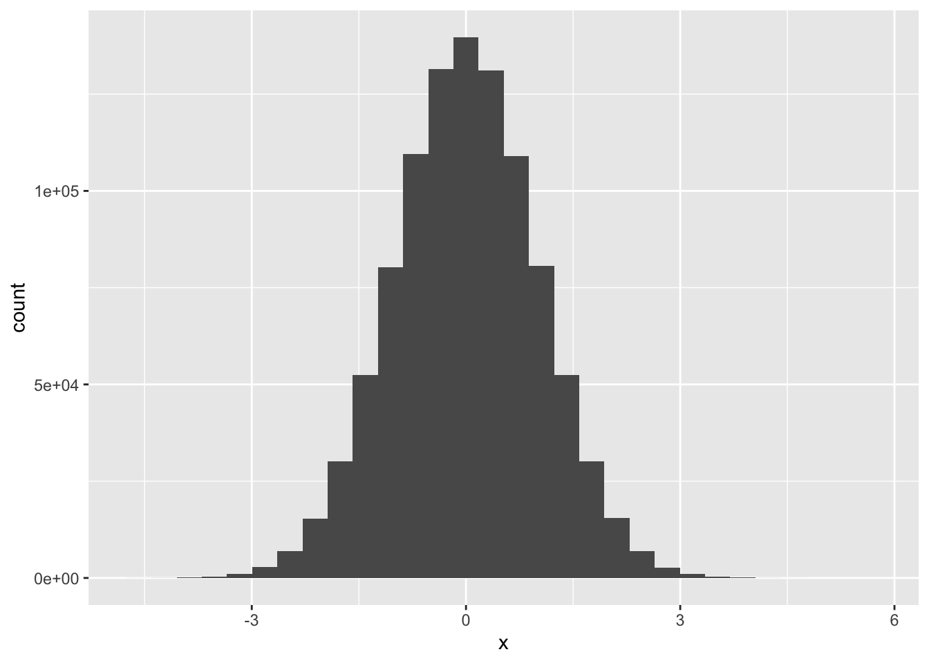
In this brief tutorial, we will explore how to estimate parameters for a normal distribution given observed and censored data. Censored data is encountered in many fields, including environmental science, where we often have data below the method detection limit (MDL). That is generally a good thing for public health as it means the concentration of the contaminant is below a level that we can detect; however, it is a challenge for statisticians and data analysts as more sophisticated methods are needed. Here, we show how to produce these estimates using base R code and functions.
x <- rnorm(10^6)
ggplot(data.frame(x = x), aes(x = x)) + geom_histogram()`stat_bin()` using `bins = 30`. Pick better value with `binwidth`.
The negative Log-Likelihood function for a normal distribution is the negative of the sum of the log of the density function of the normal distribution.
 rMLE <- function(params, y){

   mu = params[1]
   sigma = params[2]

   return(-1 * sum(dnorm(y, mean = mu, sd = sigma, log = TRUE)))

}We use starting values kind of far away from true values to make sure the optimization converges to the right values for this easy case.
 mle0 <- optim(par = c(2,3), rMLE, y = x)
 results <- mle0$par
 print(results)
[1] -0.0004567054 1.0014860050Try with a different mean and standard deviation. Also, we start with starting values quite different to make sure the optimization converges to the right values for this easy case
 x3 <- rnorm(10^6, mean = 3, sd = 6)

 mle3 <- optim(par = c(0,1), rMLE, y = x3)

 results3 <- mle3$par
 print(results3)
[1] 2.999622 6.003805 cMLE <- function(params, y.obs, y.cens = NULL){
mu = params[1]
sigma = params[2]
obs_ll <- sum(dnorm(y.obs, mean = mu, sd = sigma, log = TRUE))
cens_ll <- sum(pnorm(y.cens, mean = mu, sd = sigma, log.p = TRUE, lower.tail = TRUE))
nll <- -1 * (obs_ll + cens_ll)
return(nll)
}We will do a loop by censoring more and more data below the MDL. The MLE estimates should deviate more and more from the observed mean and standard deviation as we censor more data.
MDL <- -1.5

p <- seq(0.1, 1, by = 0.1)

results <- list()


for (i in 1:length(p)){

  # random sample of p percent of the data
  idx <- c(1:length(x)) %in% sample.int(length(x), length(x) * p[i])

  cens_data <- rep(MDL, length(x) * (1-p[i]))
  obs_data <- x[idx]

  mle <- optim(par = c(0,1), cMLE, y.obs = obs_data, y.cens = cens_data)

  results[[i]] <- mle$par

  print(paste("mu = ",results[[i]][1], "sd = ", results[[i]][2], "censored percentage = ", (100-p[i]*100)))

}
[1] "mu = -5.3170578161404 sd = 2.99552572519583 censored percentage = 90"
[1] "mu = -3.59501563712979 sd = 2.52878645139076 censored percentage = 80"
[1] "mu = -2.62489728294855 sd = 2.22261673356226 censored percentage = 70"
[1] "mu = -1.95581674394198 sd = 1.98394025323214 censored percentage = 60"
[1] "mu = -1.45331242730463 sd = 1.78209387965581 censored percentage = 50"
[1] "mu = -1.05303517142347 sd = 1.60611252514873 censored percentage = 40"
[1] "mu = -0.72394077493318 sd = 1.44413185037906 censored percentage = 30"
[1] "mu = -0.446214181679534 sd = 1.29243989070092 censored percentage = 20"
[1] "mu = -0.207790097501129 sd = 1.14572968191933 censored percentage = 10"
[1] "mu = -0.00038899346254766 sd = 1.00118853645399 censored percentage = 0"The results seem to make sense; As the censoring decrease the MLE estimates get closer to the true values. Additionally, as the censoring increases, the mean moves farther towards -Inf, away from the MDL.
We often have to estimate parameters that are strictly positive. For example, the mean concentration on the normal scale should be non-negative or a variance parameter (e.g. Kriging variance/sill).
One trick is to estimate the log of the parameter. Our estimate is then \(exp(x)\). This way, the parameter is always positive. We could do constrained optimization, but the algorithms for unconstrained optimization are more efficient and more robust.
 rMLE_log <- function(params, y){

   mu = exp(params[1])
   sigma = exp(params[2])

   return(-1 * sum(dnorm(y, mean = mu, sd = sigma, log = TRUE)))

 }

# Simulate strictly positive log-normal data
z <- rlnorm(10^3, meanlog = 3, sdlog = 1)

mle_log <- optim(par = c(5,1), rMLE_log, y = z)

results <- exp(mle_log$par)

print(paste("mu = ",results[1], "sd = ", results[2]))
[1] "mu = 34.242936274688 sd = 50.2847072198886"print(paste("observed mean = ", mean(z), "observed sd = ", sd(z)))[1] "observed mean = 34.252169019192 observed sd = 50.2792035117329"