Building an Extensible, rEproducible, Test-driven, Harmonized, Open-source, Versioned, ENsemble model for air quality

Group Project for the Spatiotemporal Exposures and Toxicology group with help from friends 😃 🤠 🌎

Installation

remotes::install_github("NIEHS/beethoven")

Getting Started

TODO

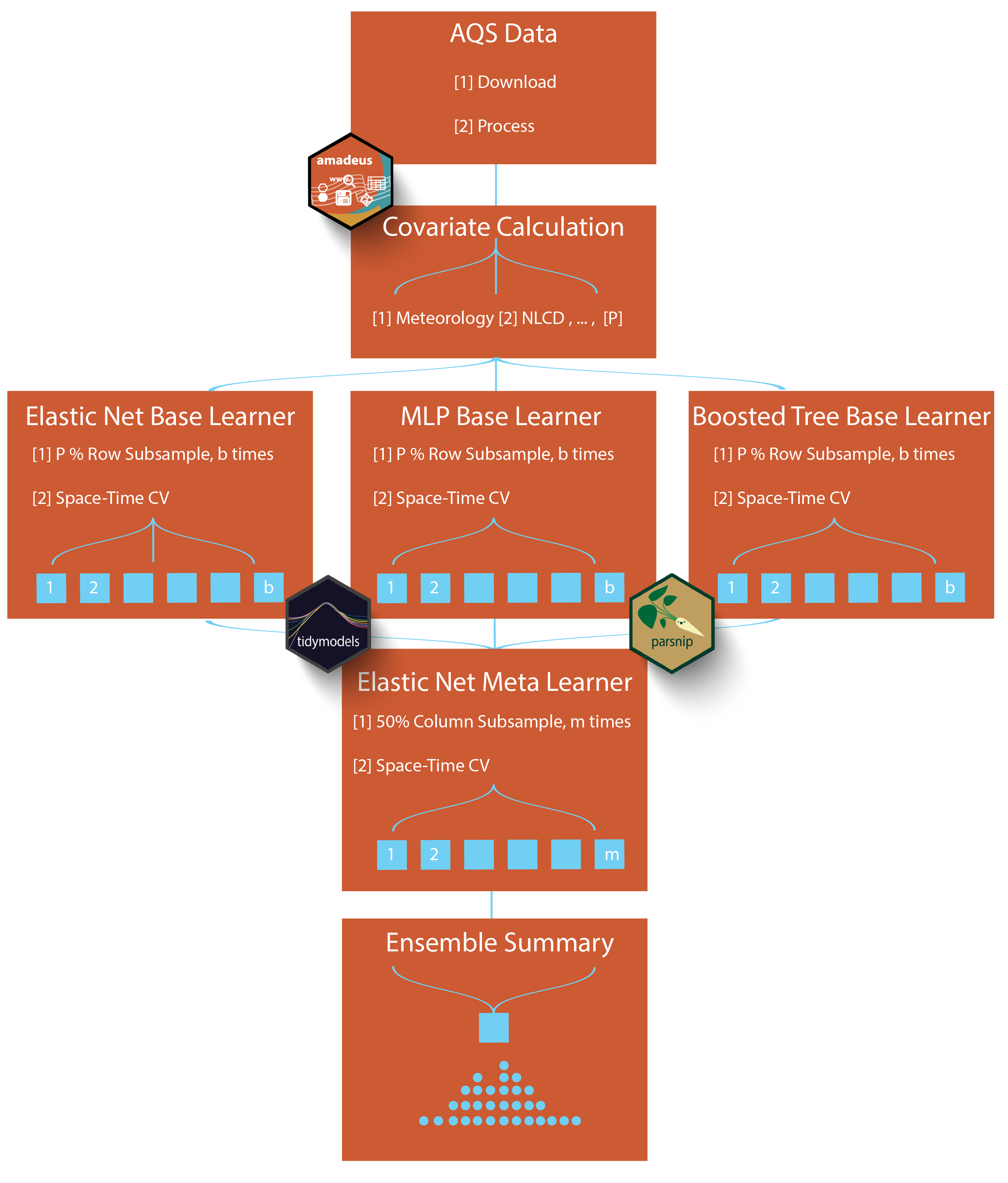
Overall Project Workflow

Targets: Make-like Reproducible Analysis Pipeline 1) AQS Data 2) Generate Covariates 3) Fit Base Learners 4) Fit Meta Learners 5) Predictions 6) Summary Stats

Placeholder for up-to-date rendering of targets

tar_visnetwork(targets)

Project Organization

Here, we describe the structure of the project and the naming conventions used. The most up to date file paths and names are recorded here for reference.

File Structure

Folder Structure

R/ This is where the main R code (e.g. .R files) lives. Nothing else but .R files should be in here. i.e. Target helper functions, model fitting and post-processing, plotting and summary functions.
tests/ This is where the unit and integration tests reside. The structure is based off the standard practices of the testthat R package for unit testing.
- testthat Unit and integration tests for CI/CD reside here
- testdata Small test datasets including our small (in size) complete pipeline testing.
- testthat.R Special script created and maintained by testthat
man/ This sub-directory contains .Rd and othe files created by the roxygen2 package for assisted documentation of R packages
vignettes/ Rmd (and potentially Qmd) narrative text and code files. These are rendered into the Articles for the package website created by pkgdown
inst/ Is a sub-directory for arbitrary files outside of the main R/ directory
- targets which include the important pipeline file _targets.R
- lookup Is a subdirectory for text file lookup table used in the pipeline to synchronize paths, names, abbreviations, etc.
.github/workflows/ This hidden directory is where the GitHub CI/CD yaml files reside

The following sub-directories are not including the package build and included only in the source code here

tools/ This sub-directory is dedicated to educational or demonstration material (e.g. Rshiny).
input/ warning soon to be deprecated This sub-directory contains data used during the analysis. It is going to be superceded by the use of targets
output/ warning: soon to be deprecated This sub-directory contains data used during the analysis. It is going to be superceded by the use of targets Currently, as of 3/29/24, the output folder contains .rds files for each of the covariates/features for model development. e.g.:
NRTAP_Covars_NLCD.rds
NRTAP_Covars_TRI.rds

Relevant files

LICENSE
DESCRIPTION
NAMESPACE
README.md

Naming Conventions

Naming things is hard and somewhat subjective. Nonetheless, consistent naming conventions make for better reproducibility, interpretability, and future extensibility. Here, we provide the beethoven naming conventions for objects as used in targets and for naming functions within the package (i.e. R/). For tar_target functions, we use the following naming conventions:

Naming conventions for tar objects. We are motivated by the Compositional Forecast (CF) model naming conventions:

e.g. [surface] [component] standard_name [at surface] [in medium] [due to process] [assuming condition] In CF, the entire process can be known from the required and optional naming pieces.

Here, we use the following naming convention:

[R object type]_[role-suffix]_[stage]_[source]_[spacetime]

Each section is in the brackets [] and appears in this order. For some objects, not all naming sections are required. If two keywords in a section apply, then they are appended with a -

Examples: 1) sf_PM25_log10-fit_AQS_siteid is an sf object for PM25 data that is log-transformed and ready for base-learner fitting, derived from AQS data and located at the siteid locations. 2) SpatRast_process_MODIS is a terra SpatRast object that has been processed from MODIS.

Naming section definitions:

R object type: sf, datatable, tibble, SpatRaster, SpatVector
role: Detailed description of the role of the object in the pipeline. Allowable keywords:
- PM25
- feature (i.e. geographic covariate)
- base_model
  - base_model suffix types: linear, random_forest, xgboost, neural_net etc.
- meta_model
- prediction
- plot -plot suffix types: scatter, map, time_series, histogram, density etc.
stage: the stage of the pipeline the object is used in. Object transformations are also articulated here. Allowable keywords:
- raw
- process
- calc
- fit: Ready for base/meta learner fitting
- result: Final result
- log
- log10
source: the original data source
- AQS
- MODIS
- GMTED
- NLCD
- NARR
- GEOSCF
- TRI
- KOPPENGEIGER
- MERRA2
- HMS
- gROADS
- POPULATION
- [Note, we can add and/or update these sources as needed]
spacetime: relevant spatial or temporal information
- spatial:
  - siteid
  - censustract
  - grid
- time:
  - daily [optional YYYYMMDD]
  - annual [optional YYYY]

Short Verion:

A shortened version for filenames is available on the punchcard at tools/pipeline/punchcard.csv

Function Naming Convenctions

We have adopted naming conventions in functions in this package as well as amadeus which is a key input package.

[High-Level-Process]_[Source]_[Object]

High-Level-Process
- download
- process
- calc
source: the original data source. Same as source section for tar objects
Object An object that the function may be acting on
- base_model
- meta_model
- feature

To run the pipeline

User settings

beethoven pipeline is configured for SLURM and is configured with defaults for NIEHS HPC settings. For adapting the settings to users’ environment, consult with the documentation of your platform and edit the _targets.R and inst/targets/targets_calculate.R (i.e., resource management) accordingly.

Setting `_targets.R`

For general users, all targets objects and meta information can be saved in a directory other than the pipeline default by changing store value in tar_config_set() at _targets.R in project root.

# replacing yaml file.
tar_config_set(
  store = "__your_directory__"
)

Users could comment out the three lines to keep targets in _targets directory under the project root. Common arguments are generated in the earlier lines in _targets.R file. Details of the function generating the arguments, set_args_calc, are described in the following.

Using `set_args_calc`

set_args_calc function exports or returns common parameters that are used repeatedly throughout the calculation process. The default commands are as below:

set_args_calc(
  char_siteid = "site_id",
  char_timeid = "time",
  char_period = c("2018-01-01", "2022-10-31"),
  num_extent = c(-126, -62, 22, 52),
  char_user_email = paste0(Sys.getenv("USER"), "@nih.gov"),
  export = FALSE,
  path_export = "inst/targets/punchcard_calc.qs",
  path_input = "input",
  nthreads_nasa = 14L,
  nthreads_hms = 3L,
  nthreads_tri = 5L,
  nthreads_geoscf = 10L,
  nthreads_nlcd = 2L,
  nthreads_narr = 24L,
  nthreads_groads = 3L,
  nthreads_population = 3L
)

All arguments except for char_siteid and char_timeid should be carefully set to match users’ environment. export = TRUE is recommended if there is no pre-generated qs file for calculation parameters. For more details, consult ?set_args_calc after loading beethoven in your R interactive session.

Running the pipeline

After switching to the project root directory (in terminal, cd [project_root], replace [project_root] with the proper path), users can run the pipeline.

[!NOTE] With export = TRUE, it will take some time to proceed to the next because it will recursively search hdf file paths. The time is affected by the number of files to search or the length of the period (char_period).

Rscript inst/targets/targets_start.R &

[!WARNING] set_args_* family for downloading and summarizing prediction outcomes will be added in the future version.